Using Multiple Hypotheses to Improve Target Tracking

If the measurement of a target's position by a surveillance radar were perfect and precise, tracking would be much easier. Changes in position would be easily converted into speed, course and accelerations, allowing motions and manoeuvres to be followed. The problem of matching tracks with measurements (the association problem) would not be the challenge that accounts for much of the complexity in a practical tracking implementation.

In the face of uncertainty and ambiguous measurements, a target tracker can use multiple hypotheses to accommodate different interpretations of the data, effectively allowing decisions to be deferred until additional information arrives.

Complexities of target tracking

The complexities of target tracking arise from the uncertainties in the measurement process associated with variations in the way radar is reflected from a target and the effects of the environment.

The accuracy of the measurement process can be reflected by the weight given to the measurement in updating the estimate of the target. This weight is represented by the filter gains (for example alpha-beta in the alpha-beta tracker, or the Kalman gains of the Kalman filter), so that a gain of 1 is an assumption that the measurement is precise, and a weight of 0 means the measurement is ignored.

A weighted measurement like this is a way of reflecting the uncertainty in the sensor data. However, it still results in a single outcome – hopefully the best outcome, but not necessarily.

The idea of multiple hypotheses in target tracking is to permit multiple outcomes to be considered. These multiple outcomes will have their own strength, so that we can still identify the best option. However, the addition of other hypotheses leaves the door open for new information to change the interpretation.

Using multiple hypotheses really just means deferring a decision until additional information makes the situation clearer.

The Association Problem

One of the key stages in a radar tracker process chain is association. This is the process of deciding how existing tracks are matched with new measurements.

In the simplest situation, an existing track may observe just a single new measurement around the expected position. We can simply associate that measurement with the track and proceed to update the track’s dynamics using some form of filter.

Even in this simple case though there are complications. For small targets in cluttered environments, we may not reliably detect the target on each update. Also, there may be spurious detections from clutter. So a single measurement for a target could be a valid measurement, or it could be that there was really no observation and what we see is spurious clutter.

We need to decide if we believe that the measurement is really derived from the target. There are problems if we get that wrong, that is ignoring the measurement if it is true, or using it if is false. Even with a simple situation, there are two possible interpretations (hypotheses).

Where tracks are close together (close being defined as a distance where the uncertainty bounds of the tracks positions intersect), there is a more interesting situation. For association, close tracks need to be considered together as a group. This group is called a track cluster.

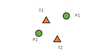
Consider two tracks and two measurements as shown in Figure 1. The tracks, T1, and T2 are close enough together so are considered as a cluster for the purposes of association. New measurements are taken in the area around T1 and T2 and these are P1 and P2. We have two tracks and two measurements. The association problem is to decide which track should be associated with, and then updated by, which measurement. For example, is P1 a measurement of T1 or of T2? We have two possibilities:

T1 is associated with P1 and T2 is associated with P2

or

T1 is associated with P2 and T2 is associated with P1

There might be other explanations of the data we are seeing, but for now we will focus on these two. These two possible interpretations of the data are two hypotheses. Since P1 and P2 are close in distance to T1 and T2 it isn’t obvious which matching is better. We can compute a figure of merit for each hypothesis based on the distance of a track to a plot for all components of the hypothesis.

Compare this to the situation in Figure2, which shows the same two tracks and two new measurements, but this time it is more obvious which associations are most likely. The proximity of P1 to T1 strongly suggests that a T1.P1 association and a T2.P2 association is much more likely than the other alternative...